
Metropolitan Area Profile and Scenario (MAPS) tool
Focussing at the spatial extent of the footprint of food production, the Metropolitan Area Profile and Scenario (MAPS) tool represents a spatial model which takes both parameters of regional yields and diets into consideration, broken down to a set of commodity groups. This allows the model’s sensitivity regarding alternative agricultural systems (conventional and organic), reduction of food loss and waste, different diets (given and health recommendations) and temperate domestic and necessary global production. The model has been applied in the five European metropolitan regions London, Berlin, Milan, Rotterdam and Ljubljana as well as for the Nairobi, Kenya. It is the main objective of the MAPS tool to develop an easy-to-adopt approach to spatially assess the necessary agricultural area to supply a pre-defined city, metropolitan area or region. It further should allow for comparative assessments of area demand for food production (based on regionalized agricultural production, diets and population data), scenario analysis of effects of organic, healthy or vegetarian diet change, prevention of food waste and loss and the regional self-sufficiency.
Modelling Procedure and Database
Food supply: The analysis of the food supply is based on actual regional agricultural conditions depending on climatic and bio-physical conditions, such as soil fertility, resulting in differences in crop yields. Therefore average values for the different commodity types are taken from agricultural statistics, mainly from regional databases, complemented by national and international figures (Statistik Berlin-Brandenburg 2012, AGRIISTAT 2012, DEFRA 2013, EUROSTAT 2012, Slovenia Statistical Office, FAO Food Balance Sheets). For crops, which cannot produced locally, such as exotic fruits, cacao, tea, coffee, etc. global yield values from FAO statistics are taken into consideration.
Livestock production: The modelling of the livestock production and fodder demand represent a specific challenge when assessing the area demand for food supply. Especially as various fodder production (on arable land) and grazing regimes are applicable, our modelling approach draws on existing area demand estimations by Woitowitz (2007) and Wakamiya (2010) for European livestock systems as well as Bouman et al. (2005) for an extension for Kenya.
Final product conversion: During the processing of food, especially in livestock production (e.g. meat, milk, eggs), but also for arable crops and fruits (e.g. sugar, cereals, fruits, beverages), there is a significant weight loss during the conversion process from the agricultural production (e.g. slaughter weight, raw milk) to the final production (etc. egg mass, edible sugar, milk, butter, cream, cheese), which is also included in the modelling exercise.
Agricultural production system: As an example of different agricultural production intensities, we have differentiated conventional production (reference system) and organic production. Therefore, the meta-analysis of Posinio et al. (2014), who have reviewed and interpreted a high number of empirical studies on yield differences between conventional and organic production. The authors found a range from in average lower yields of 19.2% to 8.5% (with multi-cropping and crop rotation) to conventional production.
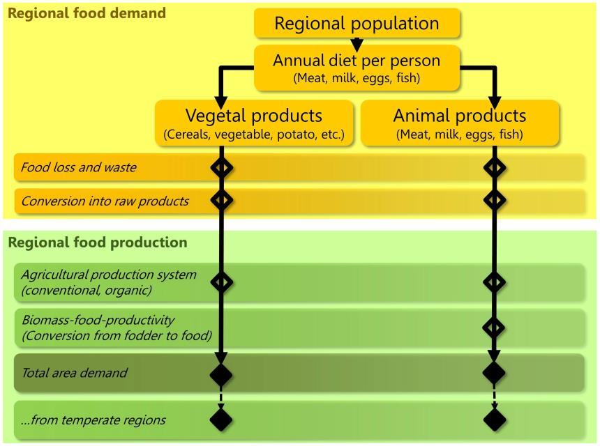
Food demand: The food demand is determined by the quantity of the regional population as well as average food consumption patterns (diets), which are also characterised by substantial differences, e.g. between countries or urban and rural areas (see Gerbens-Leenes & Nonhebel (2002)). To allow comparability between the case study regions, we applied the food balance database of the FAO (http://faostat3.fao.org/download/FB/CC/E), which covers all six regions. The basic per capita values (see table xx for the example of Berlin-Brandenburg region) is then projected for the overall regional population for the reference situation (conventional production, current food consumption and food losses and waste levels.). This will be used as starting point for the application of different scenarios of population change, food consumption, food loss and waste as well as different production intensities.
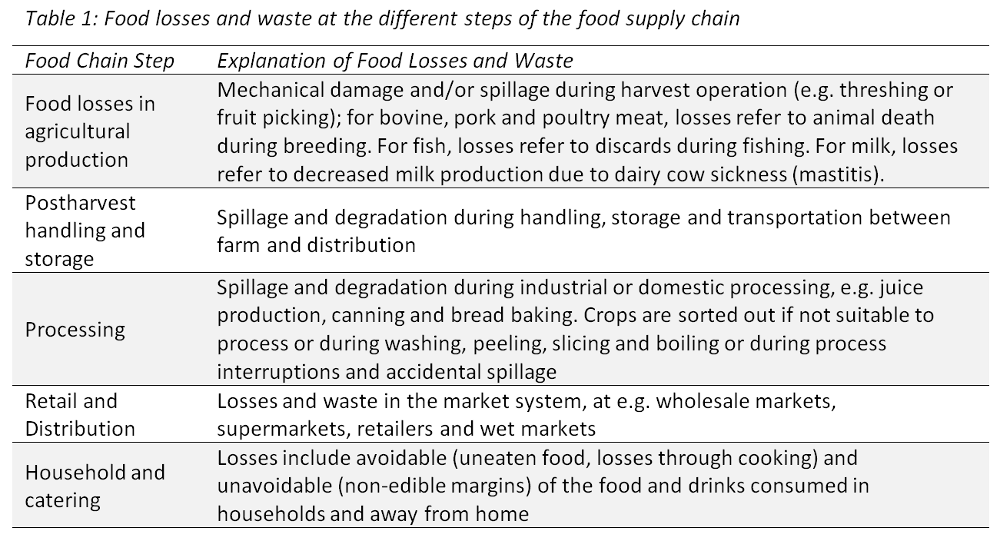
Food losses and waste: As significant contribution to food demand, the MAPS model takes the losses and waste into consideration. According to the Food and Agriculture Organisation (FAO) these losses and wastes sum up to about one third of the edible parts of food produced for human consumption, which is roughly 1.3 billion ton per year at the global scale. Consumers in Europe and North-America alone waste between 95-115 kg/year, while it is way lower in sub-Saharan Africa and South and Southeast Asia (6-11 kg/year) (FAO 2011). However, food is also lost within the whole food supply chain, including (1) Agricultural production; (2) Post-harvest handling; (3) Processing and packaging; (4) Retail and distribution; (5) Households and catering (FAO, 2011) (see Table 1). At each of the single steps a certain share of the food gets lost, avoidable and unavoidable, increasing the demand in total. By implication, food losses and waste represent the potential to reduce the food demand and therewith the agricultural area demand. There are a number of studies which aim at quantifying these shares at national, European or global scale (FAO, 2011; European Commission, 2010). In our modelling exercise, we referred to the figure of the FAO (2011) as well as Buzby and Nyman (2012). These are translated into area factors.
Spatial modeling
Starting point for the spatial modelling is the aggregated agricultural area required for food supply. This area is represented by a circle with a centre point (centroid) of the polygon of the administrative boundary. Subsequently, the radius of the circle is calculated as
,with FD (Area required for local food demand), AR (Share of agricultural area (of the region)), LT (Total area (of municipality)) and AL (Agricultural area (of municipality)). Here, the spatial model takes the available agricultural area within the municipality (AL) and the surrounding region (AR) into consideration.